In my last post I discussed how face detection works. In this post I’ll discuss how landmark detection works.

Python offers some great free libraries for face recognition. Sorry, thats a lie. They offer great wrappers for C++ libraries like dlib. Using face_recognition, we can identify the face locations of an image is as simple as face_recognition.face_locations.

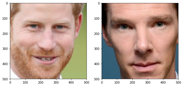
When talking about what distinguishes one face from another we normally talk about facial landmarks. For example, one person may have wide set eyes or a big nose. Identifying the location of these landmarks can help us compare faces.

Consider Prince Harry and William Cumberbatch. One defining difference between their faces is their eye width. In fact, their eyes are so distinguishing that you can probably identify each just from their eyes.

import face_recognition as fr

harry = fr.load_image_file("harry.png")
cumberbatch = fr.load_image_file("cumberbatch.png")

def crop_faces(im, size):
    """ Returns cropped faces from an image """
    faces = []
    locations = fr.face_locations(im)
    for location in locations:
        y1, x1, y2, x2 = location
        x1, x2 = sorted([x1, x2])
        y1, y2 = sorted([y1, y2])
        im_cropped = im[y1:y2, x1:x2]
        im_cropped_resized = cv2.resize(im_cropped, dsize=size)
        faces.append(im_cropped_resized)
    return faces

harry_cropped = crop_faces(harry, (500,500))[0]
cumberbatch_cropped = crop_faces(cumberbatch, (500,500))[0]

fig, axes = plt.subplots(nrows=1, ncols=2)
fig.set_size_inches(10, 10)

axes[0].imshow(harry_cropped)
axes[1].imshow(cumberbatch_cropped)

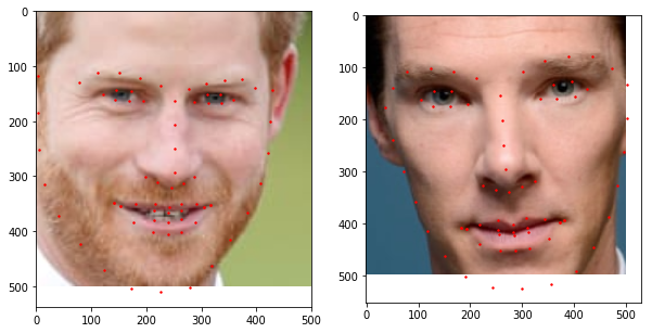
Next you have to identify the landmarks. To do that use, you guessed it, face_recognition.face_landmarks. The landmarks are calculated using Histogram of Oriented Gradients (HOG) feature combined with a linear classifier, an image pyramid and sliding window detection scheme.

def draw_landmarks(ax, im, color="r", size=2, show_original=True):
    """ Draws landmarks around an image """
    landmarks = fr.face_landmarks(im)
    xs = []
    ys = []

    for landmark in landmarks:
        for k, v in landmark.items():
            xs += [x[0] for x in v]
            ys += [x[1] for x in v]

    if show_original:
        ax.imshow(im)
    else:
        ax.imshow(np.ones(im.shape))

    ax.scatter(x=xs, y=ys, c=color, s=size)

fig, axes = plt.subplots(nrows=1, ncols=2)
fig.set_size_inches(10, 10)

harry_landmarks = draw_landmarks(axes[0], harry_cropped)
cumberbatch_landmarks = draw_landmarks(axes[1], cumberbatch_cropped)

So now we can compare the landmarks. Let’s super-impose Harrys facial landmarks to Cumberbatch:

fig, ax = plt.subplots()
fig.set_size_inches(5, 5)

harry_landmarks = draw_landmarks(ax, harry_cropped, size=8, show_original=False)
ax.imshow(cumberbatch_cropped)

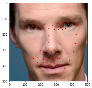
Obviously the landmarks are off, but its partially due to the two images have different rotations. Our facial detection algorithm did a good job at keeping the bridge of the nose in the same relative position, but we need to rotate the image to do a fair comparison.

Image transformations are pretty mind-bending. I found this resource to be incredibly helpful. To do affine transformations, you simply choose the operation you want, get the respective transformation matrix and perform a dot product on your original image.

For instance, the scaling, the transformation matrix is::

cx  0  0 
 0  cy 0 
 0  0  1

With cx and cy being the percentage you want to scale the x and y parameters, respectively.

Rotation is a bit most complicated, but the same principal applied:

 cosϴ  sinϴ  0
-sinϴ  cosϴ  0
 0     0     1

With ϴ being the amount in radians you want to rotate.

def transform(im, radians, translation):
    # create combined tranformation matrix
    s = np.sin(radians)
    c = np.cos(radians)
    x,y = translation

    T_r = np.array([[c, s, 0], [-s, c, 0], [0, 0, 1]])
    T_s = np.array([[1, 0, 0], [0, 1, 0], [0, 0, 1]])
    T_t = np.array([[1, 0, x], [0, 1, y], [0, 0, 1]])
    T = T_r @ T_s @ T_t
    T_inv = np.linalg.inv(T)
    
    max_dim = int((y**2 + x**2) ** 0.5) + 1

    y, x, _ = im.shape
    max_dim = int((y**2 + x**2) ** 0.5) + 1 + max(translation)
    # 2x scaling requires a tranformation image array 2x the original image
    im_transformed = np.zeros((max_dim, max_dim, 3), dtype=np.uint8)  
    for i, row in enumerate(im):  
        for j, col in enumerate(row):
            pixel_data = im[i, j, :]
            input_coords = np.array([i, j, 1])
            i_out, j_out, _ = T @ input_coords
            im_transformed[int(round(i_out)), int(round(j_out)), :] = pixel_data
    im_transformed_cropped = im_transformed[:y, :x, :]
    return im_transformed_cropped

cumberbatch_transformed = transform(cumberbatch_cropped, 0.1, (0,0))
plt.imshow(cumberbatch_transformed)

A natural product of the transform is small gaps due to the transform. The easiest way to address that is to use the nearest algorithm to fill those black gaps in, but I won’t implement that in this post.

Now if we compare the landmarks, it’s a little bit closer.

Now we can tell that the most striking difference may not be just his eyes, but his nose is also considerably longer and his face is wider.

How Facial Recognition Actually Works

We essentially transformed someone’s face into a numerical representation of points (landmarks). The logical next step to facial recognition would be to compare these landmarks and calculate some kind of landmark distance. But these are just the landmarks that make sense to humans. They may not be that distinguishing, or there may exist some other landmarks that are more distinguishing. So while this technique is useful in capturing different parts of a person’s face, they may not be best suited to tell us definitively whether two photos contain the same person.

Modern machine learning techniques do a similar process of converting a face into a numerical representation. Saying you have a large value in point 61 of your 128 point facial vector representation may not mean anything to us. After we have a numerical representation of the face, we can now use Euclidian distance to measure how different the vector is from some previous vector.

There is no magical distance that we could use to tell us that two people are the same. We can only measure distances and test their accuracy. For instance, at a distance of 0.5, what percentage of test examples are correct? Packaged facial recognition services often provide the distance as a confidence. The dlib model has a purported 99.38% accuracy on the standard LFW face recognition benchmark using a distance of 0.6.

In the next post I’ll talk about model accuracy and how well the matching algorithm works as a subject ages.