Much has been written about facial recognition and its role in society. As with a lot of topics concerning artificial intelligence, it is often discussed with an air of mysticism, as though all the all seeing machines can now peer into our souls. Depending on the narrative of the piece, its accuracy is chillingly accurate or appallingly inadequate for use. Amazon got flack for pitching their Reckognition service to law enforcement, San Fransisco banned the technology, and it has even been called racist. But the technology behind facial recognition isn’t that complicated to understand and is quite interesting.

I’m planning on writing a series of posts about the technology behind facial recognition. This post will primarily deal with facial detection.

How Facial Detection Works

Below are the libraries I’ll be using:

import cv2
import matplotlib.pyplot as plt
from PIL import Image
import numpy as np

from skimage.feature import hog
from skimage import data, color, exposure

The first step to facial recognition is, unsurprisingly, to recognize the face. How do you identify a face? Well, a face generally has two eyebrows, two eyes, a nose, a mouth and a jaw-line. So essentially like this:

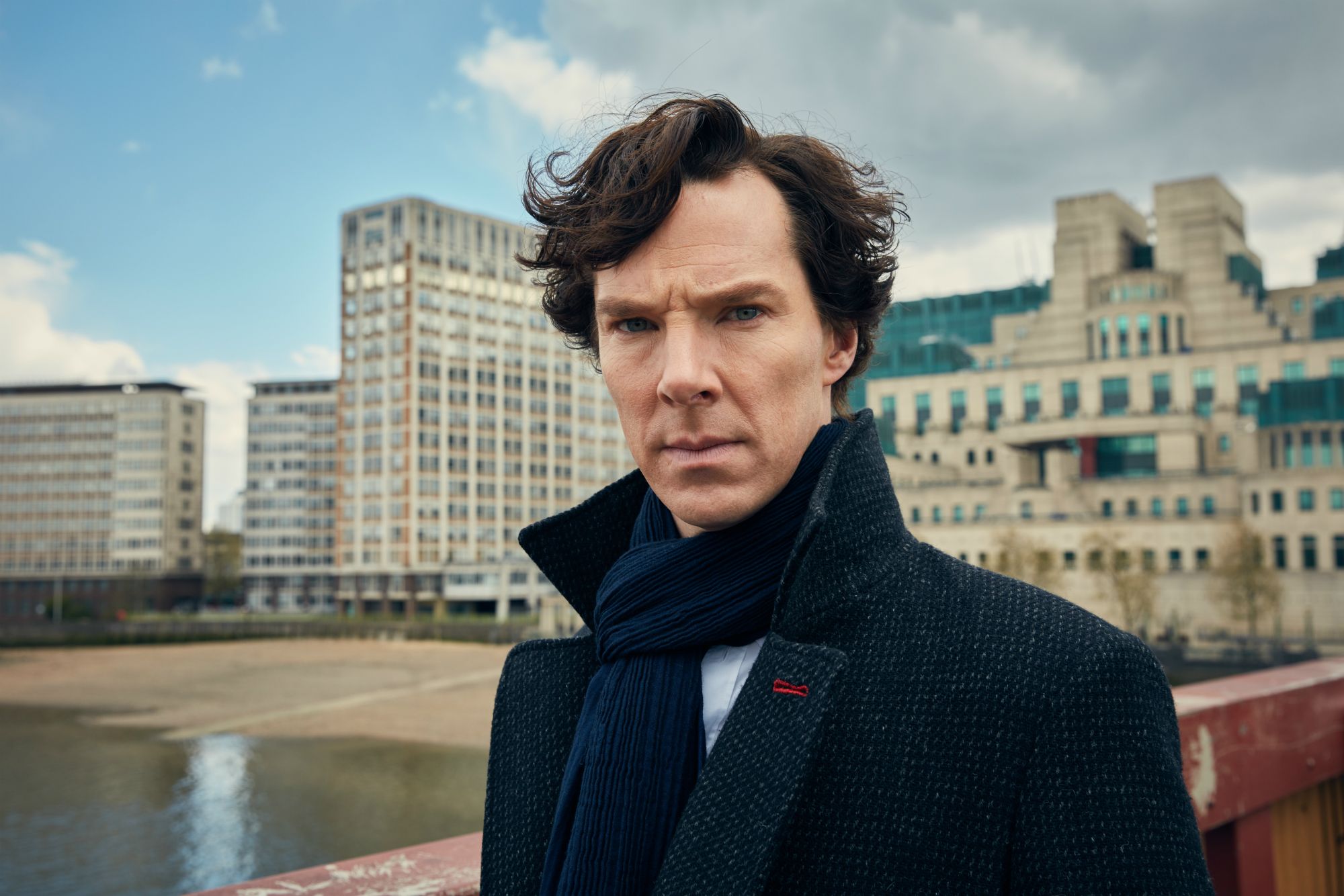
The problem is that most images have too much stuff going on. Consider Benedict Cumberbatch.

By just eyeballing it, we can make a generic face fit over Cumberbatch.

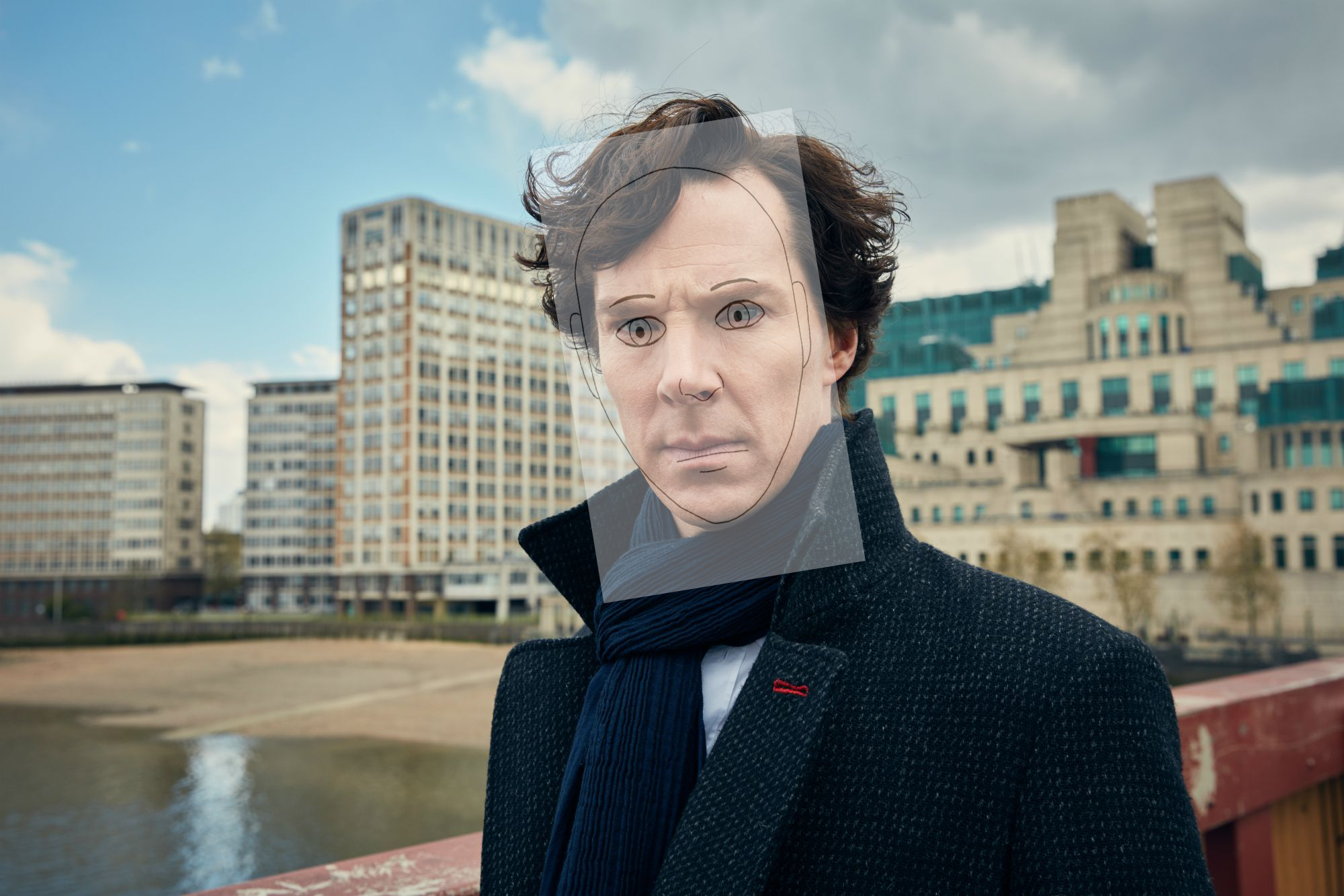
The problem is we got too much stuff going on in the picture. Sure we can eyeball it, but it would be difficult to specify a computer to match the face.

We really care just about the edges, and edges are defined by changes in gradient. We can use the Sobel operator to calculate the vertical and horizontal derivatives. Basically it’s looking any drastic change in the surrounding pixels, which is basically an edge. If one pixel is white, and the neighbor is black, then the derivate (amount of change) between the two cells would be high.

cumberbatch = Image.load("images/orig/cumberbatch.png")

gx = cv2.Sobel(cumberbatch, cv2.CV_32F, 1, 0, ksize=1)
gy = cv2.Sobel(cumberbatch, cv2.CV_32F, 0, 1, ksize=1)

gx and gy have the same shape of the original image except with the derivative in relation of its vertical and horizontal neighbors in their place.

def normalize(a):
    return (a - np.min(a))/np.ptp(a)

fig, axes = plt.subplots(ncols=3)

fig.set_size_inches(15, 10)

axes[0].imshow(normalize(gx))
axes[0].set_title("gx")

axes[1].imshow(normalize(gy))
axes[1].set_title("gy")

axes[2].imshow(normalize(gx))
axes[2].imshow(normalize(gy))
axes[2].set_title("gx & gy")

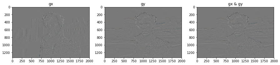
You can see that gx picked up mostly vertical edges (e.g. hair line), while gy only picked up mostly horizontal edges (e.g. mouth).

Next we’ll want to convert the cartesian coordinates into polar coordinates. Polar coordinates allow us to better see the lines of the face in magnitude and direction. We can calculate the magnitude and angle of the points directly using cv2.cartToPolar.

mag, angle = cv2.cartToPolar(gx, gy, angleInDegrees=True)

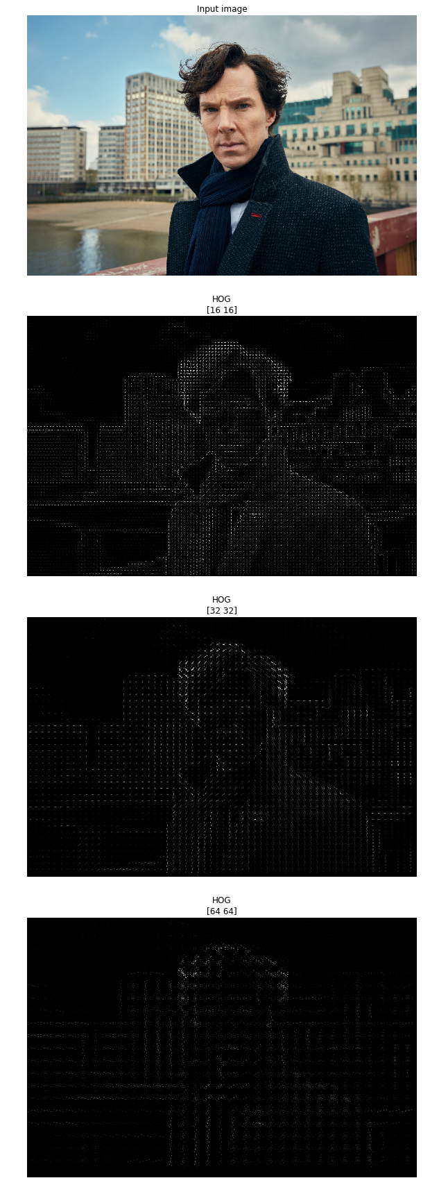
But using polar coordinates on each pixel provides too granular of a view to be used for comparison. We need to pool the polar coordinates, kind of like performing a survey of the surrounding coordinates to get a general sense of the directions each group of cells is pointing. That’s called Histogram of Oriented Gradients (HOG).

To visualize, we can plot the arrows. The number of neighboring cells we pool together will give us different levels of granularity.

fig, axes = plt.subplots(nrows=4,ncols=1, figsize=(12, 24))

axes[0].axis('off')
axes[0].imshow(cumberbatch, cmap=plt.cm.gray)
axes[0].set_title('Input image')

pixels_per_cell = np.array([16,16])

for ax in axes.ravel()[1:]:
    fd, hog_image = hog(cumberbatch, orientations=8, pixels_per_cell=pixels_per_cell,
                        cells_per_block=(1, 1), visualize=True)

    hog_image_rescaled = exposure.rescale_intensity(hog_image, in_range=(0, 15))
    
    ax.axis('off')
    ax.imshow(hog_image_rescaled, cmap=plt.cm.gray)
    ax.set_title('HOG\n{}'.format(pixels_per_cell))
    pixels_per_cell *= 2

plt.tight_layout()
plt.show()

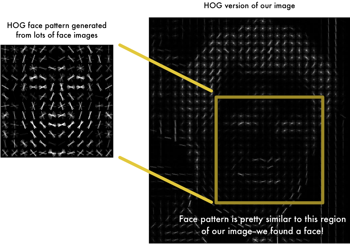
Now we’re in a good spot to actually compare to our simplified face

Well, maybe our generic face is less than ideal, but luckily there are better distillations which we can use. We can just use a sliding window to see if we get a reasonable match.

After detecting the face, we can get a lot of useful information, including location of the landmarks (e.g. nose, eyes, jawline). And it also allows us to distill the essence of a face into a vector. Comparing vectors of different faces is essentially how facial recognition works.

In the next part I’ll be discussing facial landmarks and transformations.