A generative adversarial network is a set of competing models that simultaneously learn to generate and discriminate real images from fake
In my last post post I wrote about variational auto encoders (VAEs). A VAE is composed of an encoder and decoder and can be used to compress and generate data.
In this post I’ll discuss Generative Adversarial Networks (GANs). Like VAEs, GANs are made up of two models: a generator and a discriminator and can also be used to generate data.
You can skip to the end if you just want to see the outputs, or check out my jupyter notebook.
Consider a GAN for digits. The generator portion takes random noise and tries to generate a digit that indistinguishable from actual digits. The discriminator tries to distinguish between a fake digit made by the generator and a real digit.
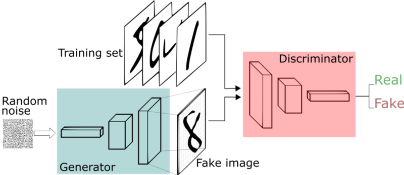
Relationship between generator and discriminator
A GAN is just a model consisting of two layers: a generator that generates images and a discriminator that tries to determine whether images are real or generated.
The crucial point is that the two models, the generator and discriminator, are linked. You can treat them independently, but that would be a lot harder to train. If un-linked ,the discriminator would just tell the generator that it either believes the image it generated is real or fake and the generator would be left on its own trying to use that to improve the images it generates.
But when the generator has access to the discriminator’s weights, it’s able to use them to build a better model to trick the discriminator. However, it cannot be allowed to do so by just messing with the discriminator’s weights. It needs to improve by changing its own weights and actually generate images that can trick the discriminator.
The downside is that since the two models are doing their own thing, the models can develop whatever method they want to do the discriminating and generating. The real goal is to have the generator generate images that can fool humans but we’re stuck with just a discriminator that we’re training along side a generator.
Building the Generative Adversarial Network
We’ll be building a GAN to generate letters (A-Z both upper and lower case). The GAN consists of a generator and a discriminator.
The Generator
Since our input is 2-dimensional, convolutional layers makes the most sense. The generator will go from some arbitrary input of 100 dimensions and return a 2 dimensional array meant to mimic a letter (28 x 28 x 1). So our input is [None, 100] and our output will be [None, 28, 28, 1].
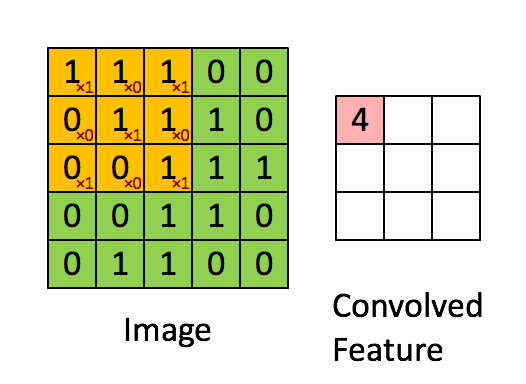
Convolutional layers consist of an n x n filter. The filter then scans a 2 dimensional array and sets the sum-product of each stride into its output. In the example below, the filter is 3 x 3, the input image is 5 x 5 with a stride of 1 and the output is 3 x 3.
Convolutional layer
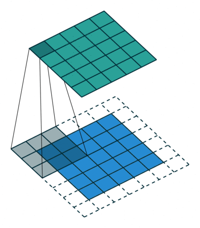
Below is another visualization of convolutional layers taken from Convolutional Arithmetic visualization. In that example, the filter is 3 x 3, the input is 4 x 4 and the stride is 1. The image is not padded so our final output is 2 x 2. Input is blue, output is green.
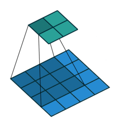
5 x 5 input, 3 x 3 filter, 2 x 2 output (input is blue, output is green)
A transposed convolution does the opposite. It goes from a filter and output to the input.
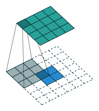
2 x 2 input, 3 x 3 filter, 5 x 5 output (input is blue, output is green)
The above examples have no padding so the input and output dimensions are different. The convolution shrinks the output (5 x 5 -> 2 x 2), while the transposed convolution grows the output (2 x 2 -> 5 x 5). But we can change the padding so that out input and output are the same dimensions. Below is the same convolution except with padding. In that case, the input and output are both the same (5 x 5). A transposed convolution would look exactly the same.
5 x 5 input, 3 x 3 filter, 5 x 5 output, padding of 1 (input is blue, output is green)
Since we want to generate an image from a flat vector, we need to use transposed convolutions. We also want to up-sample to grow our image in each transposed convolution.
Our last transposed convolution will result in the same dimension as the image we’re trying to recreate (28 x 28 x 1). We’ll apply a tanh activation to ensure our outputs are between -1 and 1. We’ll also transform our original images to be between -1 and 1 as well.
Below is the code for our generator.
def generator(img_shape, z_dim):
    inp = Input(shape=(z_dim,), name="noise")

    # Dense
    x = Dense(7 * 7 * 256, name="gen_dense")(inp)
    x = LeakyReLU(alpha=0.01, name="gen_act")(x)
    x = BatchNormalization(name="gen_batch_norm")(x)

    x = Reshape([7,7,256], name="gen_reshape")(x)
    x = Dropout(0.4)(x)
    x = UpSampling2D(name="gen_up_sample")(x)

# Transposed Convolution
    x = Conv2DTranspose(128, 5, padding="same", name="gen_conv_1")(x)
    x = LeakyReLU(alpha=0.01, name="gen_act_1")(x)
    x = BatchNormalization(name="gen_batch_norm_1")(x)
    x = UpSampling2D(name="gen_up_sample_1")(x)

# Transposed Convolution
    x = Conv2DTranspose(64, 5, padding="same", name="gen_conv_2")(x)
    x = LeakyReLU(alpha=0.01, name="gen_act_2")(x)
    x = BatchNormalization(name="gen_batch_norm_2")(x)

# Transposed Convolution
    x = Conv2DTranspose(32, 5, padding="same", name="gen_conv_3")(x)
    x = LeakyReLU(alpha=0.01, name="gen_act_3")(x)
    x = BatchNormalization(name="gen_batch_norm_3")(x)

    out = Conv2DTranspose(1, 5, padding="same", name="gen_conv_4", activation="tanh")(x)

    return Model(inp, out, name="generator")
Here’s what our generator looks like:
Layer (type)                 Output Shape              Param #
=================================================================
noise (InputLayer)           (None, 100)               0
gen_dense (Dense)            (None, 12544)             1266944
gen_act (LeakyReLU)          (None, 12544)             0
gen_batch_norm (BatchNormali (None, 12544)             50176
gen_reshape (Reshape)        (None, 7, 7, 256)         0
dropout_16 (Dropout)         (None, 7, 7, 256)         0
gen_up_sample (UpSampling2D) (None, 14, 14, 256)       0
gen_conv_1 (Conv2DTranspose) (None, 14, 14, 128)       819328
gen_act_1 (LeakyReLU)        (None, 14, 14, 128)       0
gen_batch_norm_1 (BatchNorma (None, 14, 14, 128)       512
gen_up_sample_1 (UpSampling2 (None, 28, 28, 128)       0
gen_conv_2 (Conv2DTranspose) (None, 28, 28, 64)        204864
gen_act_2 (LeakyReLU)        (None, 28, 28, 64)        0
gen_batch_norm_2 (BatchNorma (None, 28, 28, 64)        256
gen_conv_3 (Conv2DTranspose) (None, 28, 28, 32)        51232
gen_act_3 (LeakyReLU)        (None, 28, 28, 32)        0
gen_batch_norm_3 (BatchNorma (None, 28, 28, 32)        128
gen_conv_4 (Conv2DTranspose) (None, 28, 28, 1)         801
=================================================================
Total params: 2,394,241
Trainable params: 2,368,705
Non-trainable params: 25,536
The Discriminator
Our discriminator is similar to the generator except instead of using transposed convolutional layers, we’ll just be using convolutional layers. As we used up-sampling in the generator, we’ll use strides of 2 in our discriminator so we can shrink the output at each convolution.
Our final output will be a value between 0 and 1 signifying whether the discriminator believes that the image is real or fake. For that we use a sigmoid activation.
def discriminator(img_shape):
    inp = Input(shape=[*img_shape, 1], name="image")

    x = Reshape([*img_shape, 1], name="disc_reshape")(inp)

    x = Conv2D(64, 5, strides=2, padding="same", name="disc_conv_1")(x)
    x = LeakyReLU(alpha=0.01, name="disc_act_1")(x)
    x = Dropout(0.4)(x)

    x = Conv2D(128, 5, strides=2, padding="same", name="disc_conv_2")(x)
    x = LeakyReLU(alpha=0.01, name="disc_act_2")(x)
    x = Dropout(0.4)(x)

    x = Conv2D(256, 5, strides=2, padding="same", name="disc_conv_3")(x)
    x = LeakyReLU(alpha=0.01, name="disc_act_3")(x)
    x = Dropout(0.4)(x)

    x = Conv2D(512, 5, strides=1, padding="same", name="disc_conv_4")(x)
    x = LeakyReLU(alpha=0.01, name="disc_act_4")(x)
    x = Dropout(0.4)(x)

x = Flatten()(x)

out = Dense(1, activation="sigmoid", name="disc_out")(x)

return Model(inp, out, name="discriminator")
This is what our discriminator will look like:
_________________________________________________________________
_________________________________________________________________
Layer (type)                 Output Shape              Param #
=================================================================
image (InputLayer)           (None, 28, 28, 1)         0
_________________________________________________________________
disc_reshape (Reshape)       (None, 28, 28, 1)         0
_________________________________________________________________
disc_conv_1 (Conv2D)         (None, 14, 14, 64)        1664
_________________________________________________________________
disc_act_1 (LeakyReLU)       (None, 14, 14, 64)        0
_________________________________________________________________
dropout_7 (Dropout)          (None, 14, 14, 64)        0
_________________________________________________________________
disc_conv_2 (Conv2D)         (None, 7, 7, 128)         204928
_________________________________________________________________
disc_act_2 (LeakyReLU)       (None, 7, 7, 128)         0
_________________________________________________________________
dropout_8 (Dropout)          (None, 7, 7, 128)         0
_________________________________________________________________
disc_conv_3 (Conv2D)         (None, 4, 4, 256)         819456
_________________________________________________________________
disc_act_3 (LeakyReLU)       (None, 4, 4, 256)         0
_________________________________________________________________
dropout_9 (Dropout)          (None, 4, 4, 256)         0
_________________________________________________________________
disc_conv_4 (Conv2D)         (None, 4, 4, 512)         3277312
_________________________________________________________________
disc_act_4 (LeakyReLU)       (None, 4, 4, 512)         0
_________________________________________________________________
dropout_10 (Dropout)         (None, 4, 4, 512)         0
_________________________________________________________________
flatten_2 (Flatten)          (None, 8192)              0
_________________________________________________________________
disc_out (Dense)             (None, 1)                 8193
=================================================================
Total params: 4,311,553
Trainable params: 0
Non-trainable params: 4,311,553
The Generative Adversarial Network
Since the generator output is the same as the discriminator input, we can just connect the two to form the GAN.
def generative_adversarial_model(img_shape, z_dim):
    gen = generator(img_shape, z_dim)
    disc = discriminator(img_shape)

    inp = Input(shape=(*gen.input_shape[1:],), name="image")
    img = gen(inp)

    # NOTE: We do not want the discriminator to be trainable
    disc.trainable = False

    prediction = disc(img)

    gan = Model(inp, prediction, name="gan")
    gan.compile(loss="binary_crossentropy", optimizer="adam", metrics=["accuracy"])

    return gan
The important thing to note is that when we combine the two, we have to make sure the discriminator is not trainable. We don’t want the generator to improve just by messing with the discriminator’s weights.
Here’s what the final GAN looks like:
_________________________________________________________________
Layer (type)                 Output Shape              Param #
=================================================================
image (InputLayer)           (None, 100)               0
_________________________________________________________________
generator (Model)            (None, 28, 28, 1)         2394241
_________________________________________________________________
discriminator (Model)        (None, 1)                 4311553
=================================================================
Total params: 6,705,794
Trainable params: 2,368,705
Non-trainable params: 4,337,089
Training the Generative Adversarial Network
Unrealistic Generator Output
Training a GAN is tricky for a number of reasons. As mentioned earlier, the discriminator will do its own thing in determining whether an image is real or not. So its important to look at the output periodically to make sure its in line with what we think a real image looks like.
Mismatch Between Generator and Discriminator
Another issue is that checking whether an image is real or not (discriminator) is a lot easier task than generating a valid looking image from random input (generator). So there’s naturally a mismatch between the generator and discriminator. To address that, we can do several things. One is to make the generator more powerful than the discriminator. The other thing we can do is to train the generator more than the discriminator.
While we’re training, it’s helpful to see how the generator and discriminator is doing in relationship to each other. We want them to be roughly equal strength during training and train the simultaneously. We’ll switch between training the generator and the discriminator.
We can put in a criteria to say the generator / discriminator is good enough before we move on to train the discriminator / generator.
Practically speaking, the generator can never get above 50% because if the discriminator was wrong more often than not, it could just simply switch its output to predict the opposite and attain a higher accuracy.
For the same reason, the generator can’t get above 50% accuracy. Let’s say good enough is 20% validation accuracy for the generator and 50% validation accuracy for the discriminator.
Proportional Representation of Different Characters
Another problem is that our generator can just learn to create one type of character indistinguishable from actual input. This isn’t that big of a problem since our discriminator can just call all those fake and still do fairly well even though it would be mislabeling a large number of real images. But ignoring classes and distributions as we’ll do does not guarantee out generator will be able to generate all possible characters. It just maps a random input to just about any output that resembles a letter. It’s a bit surprising the amount of diversity we get in the end.
Training
Below is the training function we’ll use. It’ll switch between training the GAN, which is essentially just training the generator portion. The input will be a random vector and it will try to fool the discriminator into thinking its real. Remember that we made the discriminator portion of the GAN un-trainable. We’ll then train the discriminator separately.
Results
After 1 epoch, we can see the generator is not exactly outputting random noise, but its certainly not a character. Above each image, we can see the discriminator’s output for that particular image. A score of 1.0 means the discriminator is 100% sure its a real image while a score of 0.0 means it thinks there’s a 0% chance of it being real.
Gen status: val_loss: 0.69608 val_acc: 0.25000 loss: 0.70158 acc: 0.39844 epochs: 4.
Disc status: val_loss: 0.18264 val_acc: 0.96875 loss: 0.35883 acc: 0.83594 epochs: 2

1 iteration
One thing to note is that the number of batches we used to train the generator was 4 compared to 2 for that of the discriminator. The final validation accuracy was 25% and 97% for the generator and discriminator, respectively.
As a side note, gen status is collected immediately after the generator is trained, so the actual generator accuracy at the end of the iteration is lower since the discriminator has been trained at the time the statistic was calculated.
Iteration 2 is similar but we can see the generator is getting better at tricking the discriminator. This back and forth is common when training GANs.

2 iterations
By the 25th iteration, we can see something sort of resembling letters. We can also see that we trained the generator on 51 batches while only training the discriminator for 36 batches. Despite that, the accuracy on the discriminator is 68%.
25 iteration.
Gen status: val_loss: 0.86473 val_acc: 0.50000 loss: 0.91149 acc: 0.40625 epochs: 51
Disc status: val_loss: 0.81117 val_acc: 0.68750 loss: 0.53552 acc: 0.74219 epochs: 36

25 iterations
After 500 iterations, the generator is looking somewhat more convincing.

500 iterations
Let’s review more output values of the generator in comparison to actual images. Again, the percent probability that the discriminator places on the image being real is above the image. Green titles mean the image is in fact real, while red means the image is generated.

500 iterations
So we’re going in the right direction although we’re not there yet. The discriminator is still doing a fairly good job and although the generators output is somewhat believable, some images don’t actually resemble characters, just images generated using similar lines. We should continue training.
After 5,000 iterations, the output is more convincing.

5,000 iterations
The output of the generator is considerably better. The discriminator is still correctly marking almost all of the fake images as fakes, but it’s getting a lot of false positives as well. And most importantly, a significant portion of the generated images look as though they are real, at least to me.
Next Steps
GANs are incredibly useful but notoriously difficult to train. There has been a lot of work done with stopping criteria and better loss functions. Wasserstein GAN (WGAN) and the WGAN-Gradient penalty are objectively better to our model, but they share the same basic structure. I may write my own implementation of WGANs in a future post, or you can see the Keras implementation.
The other difficult part is finding the right model structures, but that’s a common problem in all of machine learning. What makes GANs particularly annoying is that you cannot rely simply on the loss function in determining whether a model structure is suited to the task. But you have to continuously monitor the output. Depending on what you’re training, there may be some ways around it, but in general monitoring the output is a big part of creating useful GANs.
By Branko Blagojevic November 5, 2018