Variational Auto Encoders are simpler than they appear and are the building blocks of generative models
Variational Auto Encoders are used to learn probability distribution function of images. By viewing their latent space we can see what’s really going on and use it to generate our own examples
I have read a fair number of posts about variational auto encoders but only recently did I try my hand in generating my own. I’ve been going through the early access edition of GANs in Action by Manning.
An auto-encoder deconstructs (or encodes) some data into a hidden representation with the goal of losing as little information as possible. Its performance is measured by how well it can reconstruct (decode) the data based on its internal representation.
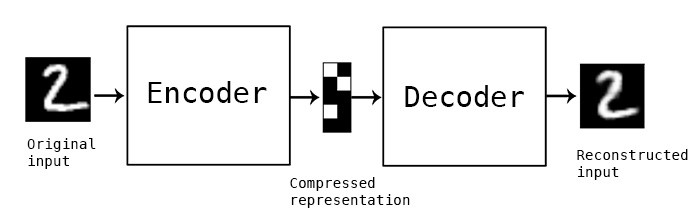
The cool thing about auto-encoders is that they are unsupervised. Nowhere in the example above did we tell the encoder the number is a 2. So we can use them to create a structure on a data set without the need for labels. We can then use that structure for supervised training. We also don’t tell it how to encode the data. We just provide a structure for the encoder and decoder, and measure how well its doing based on how much information is lost in the process.
A variational auto-encoder (VAE) is an auto-encoder, except instead of learning a compressed representation, it learns a probability distribution of the data:
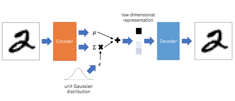
This is the point at which most explanations get all hand-wavy and spill a few words about latent space. But all this means is that the compressed representation will be a mean and standard deviation, representing a normal distribution. When we connect it to the decoder, we’ll want to take a noise sample using the mean and variance. This is the μ + Σ * ε from the graph above. This just means that when we decode, we’ll use the mean and add the standard deviation multiplied by some random normal value.
def sampling(args):
    z_mean, z_log_var = args
    epsilon = K.random_normal(shape=(latent_dim,), mean=0.0)
    return z_mean + K.exp(z_log_var/2.0) * epsilon
The other interesting thing about auto-encoders is that you can inject your own values into the process and generate output. From there you can map out a latent space and see the internal representation of our model.
Implementation
Most posts use the mnist handwritten numeric digit data set but we’ll use emnist, the handwritten character data set instead. Someone on Kaggle conveniently transformed the dataset into a csv. I’ve excluded some function definitions. My full code can be found here.
%matplotlib inline
import imageio
import matplotlib.pyplot as plt
import numpy as np
import pandas as pd
from PIL import Image
train = pd.read_csv("emnist-letters-train.csv", header=None)
test = pd.read_csv("emnist-letters-test.csv", header=None)
mappings = {}
with open("emnist-letters-mapping.txt") as f:
for line in f.readlines():
code, lower, upper = line.split()
mappings[int(code)] = chr(int(lower))
def display_images(imgs, names, max_imgs=100):
""" Displays images and their corresponding names"""
...
def process_emnist(arr, mappings):
""" Process emnist letters """
...
X_train, y_train = process_emnist(train, mappings)
X_test, y_test = process_emnist(test, mappings)
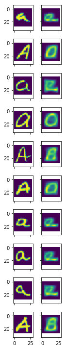
display_images(X_train[:10],y_train[:10])
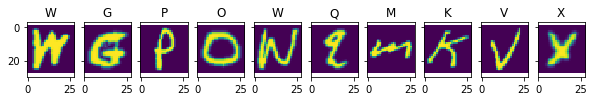
Our training set is (88800, 28, 28) representing 88,800 letters from A to Z in either upper or lower case.
Below we create the VAE.
A variational auto encoder is just an encoder that feeds a decoder and encodes to a probability density function. We define the models independently and then define the VAE as the combined model. The function returns two models: one for training and one for evaluation. The only difference is that for training, the final layer is hooked up to the sampling layer. But when we want to display our results, we should not include the noise. That model is vae_eval and is just connected to the z_mean layer.
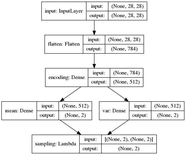
The final layer of the encoder is the sampling layer which we defined ourselves and wrapped in a Lambda layer. The mean and var layers are used for the loss function which tracks how far away our probability distribution in our encoding is from a mean of 0 and a standard deviation of 1. The mean layer is also used when we want to see our results.
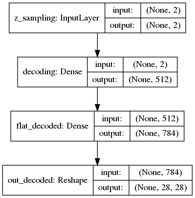
Decoder
The decoder is relatively straight forward. It takes an input of 2 representing our latent dimensions. It then reconstructs the image.
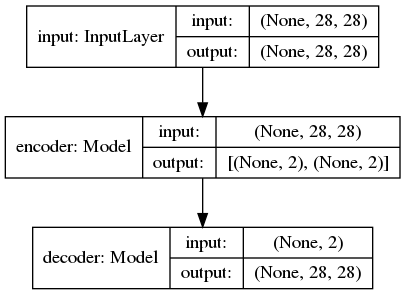
Variational Auto Encoder
The VAE is just the two combined. Note that the encoder returns both the mean latent value and a noisy sampling of the latent space. We’ll train on the noisy model and display our results on just the mean.
All that’s left is to fit the model.
vae_train.fit(
    X_train,
    X_train,
    shuffle=True,
    epochs=epochs,
    batch_size=batch_size,
    validation_data=(X_test,X_test),
    verbose=1,
    callbacks=[EarlyStopping(patience=4)]
    )
Let’s see how it did.
Not great. The problem is that our representation isn’t deep enough. Ideally we would want to use convolutional layers to get a deeper understanding of the letters and edges.
Let’s see how the latent space looks. We can do so by getting the decoder and feeding it a series of values and seeing what it comes up with. To get the encoder and decoder, we can just reference the second and third layers of the VAE.
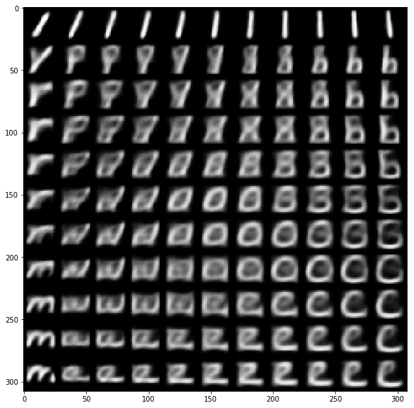
Latent space
It looks crowded. There is some semblance of Ms in the bottom left and Is in the top right. By comparison, here’s how the same analysis looks on numeric digits:
Latent space of a VAE trained on digits
In the latent space you can see something representing nearly all the digits. However, the VAE is still having some trouble distinguishing between 4s, 7s and 9s due to their similarity in shape.
We can increase our latent space by adding more latent dimensions (currently 2). However if we go above 2 layers, we lose the ability to easily represent the latent space as a grid. The other way is to limit our training set to just a subset of the original set. Below I train the vae only on the vowels.
def filter_char(X, y, chars):
    if type(chars) is not list:
        chars = [chars]
    idxs, chs = zip(*[(idx, ch) for idx, ch in enumerate(y) if ch in chars])
    return X[np.array(idxs)], chs

X_train_vowels, y_train_vowels = filter_char(X_train, y_train, ["A","E","I","O","U"])
X_test_vowels, y_test_vowels = filter_char(X_test, y_test, ["A","E","I","O","U"])
This is much better with a clearer distinction between each vowel, although the model does get some letters confused.
The next step would be to build a bigger model ideally one using convolutional layers, which is the more natural way to represent images. Another option would be to increase our latent space dimensions. We’re currently using only 2 dimensions and the nice thing about that is that we can represent the output in a 2d grid to evaluate. But more dimensions would allow for a richer representation and better performance.
By Branko Blagojevic on October 25, 2018