This is a continuation of my series on reinforcement learning. I’d recommend the second post if you’re unfamiliar with OpenAI and the third…
This is a continuation of my series on reinforcement learning. I’d recommend the second post if you’re unfamiliar with OpenAI and the third post if you’re unfamiliar with using neural networks to train a policy. This borrows some code and ideas from Arthur Juliani’s post, especially the game environment.
All the code below is available on my github tutorial on reinforcement learning, specifically Part 4 — Deep Q-Networks and Beyond with Keras or Part 4 — Deep Q-Networks and Beyond with Tensorflow for you sadists out there.
In this post, we’ll use Q-learning to indirectly determine policy. This method was made popular in 2013 when a DeepMind showed Q-learning to be successful in solving a number of Atari games from analysis of the pixel values.
Q-learning is a model free reinforcement learning technique. Model free means we learn directly from the environment and don’t build out a model to learn how an environment works. We just learn from the observations.
The Q network lookup can be seen below:

And to update the value, we just take the old value, and nudge it a little bit based on what we thing the new value is.

Because everything we’re doing is approximation and dynamic, we use a small learning rate to guide our network to the optimal values.
Q-learning is basically an indirect method used to determine policy by looking up how good a certain state-action pair is. The state is just a representation of the game environment. It can be anything (speed, life, coordinates, or in our case raw pixels). Action is just your available actions from that state (move left, right, etc). Reward is provided by the game environment or determined by us based on what we’re trying to do. If we’re playing Mario, we might want the reward to be distance from start, coins collected or some other game statistic.
Consider a simple one-dimensional environment where we’re a robot and we can move left or right. Our state may look like this:

What’s our Q-network look like?
Q([-1, 🤖, 1], left) = -1
Q([-1, 🤖, 1], right) = 1
Simple enough. A left move will get us -1 reward, right move gets us 1 reward. So if you used this Q-network and you saw state [-1, 🤖, 1], you would look at the possible rewards and just pick the highest one (right). In actuality, we may want to setup are Q-network like this:
Q([-1, 🤖, 1]) = [-1, 1]
The -1 in the 0 index means action 0 (left) yields a -1 reward, while action 1 (right) yields a +1 reward.
That’s just for one step, but suppose you want to consider more steps.

Our one step Q-network still looks the same, but we want to consider two steps so we have to consider what happens after that initial step:
Q(s,a) = reward + discount_factor * max(Q(s(t+1),a)

One step:
Q([10, -1, 🤖, 1, 1], left) = -1
Q([10, 🤖, 0 , 1, 1], left) = 10
Q([10, 🤖, 0 , 1, 1], right) = 0

Q([10, -1, 🤖, 1, 1], right) = 1
Q([10, -1, 0 , 🤖,1], left) = 0
Q([10, -1, 0 , 🤖,1], right) = 1

Two step:
Q([10, -1, 🤖, 1, 1], left) = -1 + max(10, 0) = 9
Q([10, -1, 🤖, 1, 1], right) = 1 + max(1, 0) = 2
As you can see from above, although going left is the worse option (-1 immediate reward), it leads to a state that is worth 10 points (going left again).
A few things to note. We prefer rewards now versus rewards in the future. So we apply a discount factor to the future rewards. That’s why the formula is reward + discount_factor * future_reward. This is a hyper-parameter we’ll have to set during learning. Set too low, bots will act too greedily and not plan well. Set too high, bots will sometimes unnecessarily delay moves or act with too much confidence as to the future reward.
Also since considering future steps can quickly spiral out of control in terms of the state space to explore, we need to bootstrap. What that means is that we can’t look too far ahead so we’ll rely on some estimate of the final state and use that. Besides, when we’re learning, we’re just making small steps towards what we believe to be the optimal solution.
To bootstrap, research has shown that it makes sense to use another network to determine the q-values to learn. The target network is the one you’re using to bootstrap q-values and the main network is the one you’re training and using to determine policy. You never train the target network but periodically you update the weights of the target network with those of the main network. Here’s the full algorithm for the mathematically inclined. Note the θ is the main network and θ ̅ is the target network.
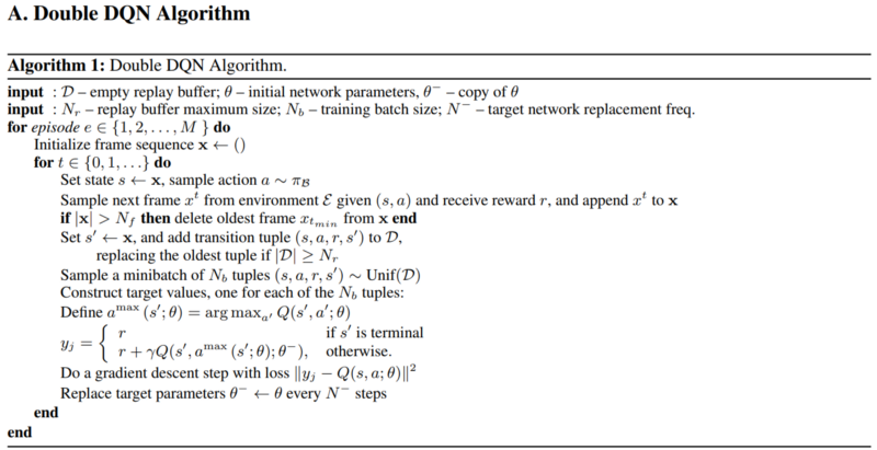
So to summarize, a Q-network maps a state and action pair to it’s expected value. We can use a state, and look at the action options and determine what action would lead to the best results. To train the network, we take the state and action pair we had observed and map it to the immediate reward plus what we believe the next state is worth.
Before we begin talking about implementing a Q-network, let’s discuss the environment briefly. This was originally thought up by Arthur Juliani in his post on Q-networks.
Our environment consists of an rgb array of shape (84,84,3). We play as the blue square, and move left, right, up or down (4 actions) and try to collect the green squares (+1 reward), while avoiding the red squares (-1 reward).
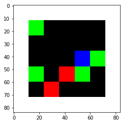
So our state is (84, 84, 3) and our actions are 4. We want some function that takes a state and outputs 4 values, one for each action.
We’ll build our bot to consider the raw pixels. This makes the challenge considerably harder because our bot will have to learn low level concepts like edges and distinguishing between the different colors and shapes. Also, we have a static point of reference with only the blue square moving. So it won’t be as simple as if green to the left, move left.
We will learn from pixel values without any input other than the raw rewards we had discussed earlier. We’ll just have the bot act randomly, update the network, act a little smarter based on what we observed, and learn from that. Rinse and repeat.
One way to learn from image data is to use convolutional layers. Convolutional layers are a bit beyond the scope of this post, but I’ll try to describe them in a high level.
What convolutional layers do is create a filter (e.g. 3 x 3) and do a dot product on every value of the image to come up with a new set of value.
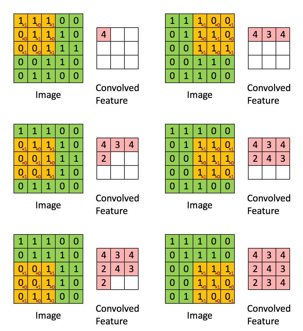
The idea is that a filter would be able to detect simple geometric patterns. And when you apply a convolutional layer on top of a convolutional layer, it can detect more and more complex features such as circles, squares and eyes. Some of the best image detection software is simply a series of convolutional layers on top of each other and a final dense layer at the end.
So we have these convolutional layers stacked on top of each other. Then we’ll want to break out the value and advantage values. The value is the reward of the current move. The advantage is the the value from that future state. So in our case Q([10, -1, 🤖, 1, 1], left), our value would be -1 and our advantage would be [10, 0]. Then we add the value to advantage for our final Q-value. In our example the final Q-value would be -1 + [10, 0] = [9, -1]
Below is the network class and what the network will look like.
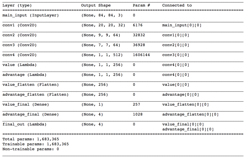
This nice thing about using a neural-network is that it is pretty well encapsulated. We can add or remove layers, add regularization, add frame augmentation, or plug in a totally different kind of network. It will work as long as the top layer accepts (84, 84, 3) and outputs a value of 4 (4 actions available). So feel free to experiment.
Another concept that will help with learning is the idea of an Experience Replay. It’s just an object that stores experiences (game replays). When we want to train from the network, we take a sample from the trove of experiences we have collected. Eventually we cycle out older experiences for newer ones, since the newer experiences are likely more relevant to actual game play based on our current network. Below is an implementation of experience replay:
We’ll periodically pull some experiences from the experience replay, train our network a bit, and continue playing using the updated network. An experience sampled from the experience replay will hold [state, action, reward, next_state, done].
Train batch is [[state,action,reward,next_state,done],…]
train_batch = experience_replay.sample(batch_size)
Separate the batch into its components
train_state, train_action, train_reward,train_next_state, train_done = train_batch.T
We then use our target network to determine what we think the values should be based on the state and action. Below is a snip of how the training works.
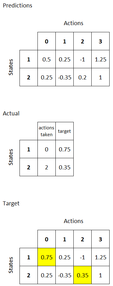
Since we’re only updating the actions we took, the easiest way to do that is to predict what the model will output anyway, and update those actions that we took. The other actions will not be updated since they’ll tie out exactly with what the model predicted (loss of 0). It’s not very efficient since we have to predict everything from the model but I think it’s the most straight-forward way.
Below is an example of how we’re updating our values:
The best part is looking at what your bot learned. It usually results in a few head-scratchers and a deeper understanding of what the network is learning. Here is the output of 50 steps from a bot I trained (follow the blue square):
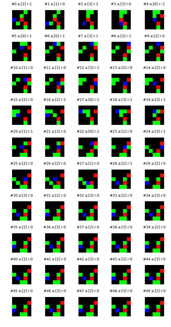
The bot isn’t perfect but it does pretty well to scoop up the green squares. However on step 3, it doesn’t go around a red square. Let’s take a closer look:
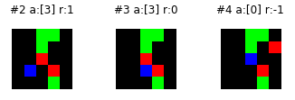
My guess is that on step 2, it compared the right square to the up square. It likely thought the right square was more valuable since it’s closer to the square below it and the cluster of squares above it. So it took the shortcut through the red square. Probably not ideal. It could go away with more training. Or another thing you may want to do is replicate the environment, feed it into the network and see what’s really going on. If the right and up actions are very similar, perhaps more training is required. You can just train it on this edge case. In future posts I’ll speak a bit about choosing more meaningful training examples and analyzing the behavior of the bot.
Another common thing you may see is an endless loop. Below is an example.

My guess is that the bot is torn between two events. It goes for the left square but then immediately before capturing the square, it is drawn by the three other squares to the right. In a future post we’ll use an recurrent neural net to provide our bot with a memory. In that case it will “remember” that it was going for the left square and (hopefully) capture it. Another option is to use a non-deterministic policy. So if the Q network has rewards of [0.51, 0.49], it won’t necessarily choose the 0.51 every time.
In summary, Q-networks map a state and action to an expected future reward. We setup a Q-network to accept a state, run it through some convolutional layers and determine the value of each state-action pair. We’ll play the game making random moves and record our experiences. From our experiences, we’ll train the Q-network to calculate the value of each state-action pair. From that Q-network, we can choose the actions that result in the highest state-action values, and use those values to continue to train our bot.
By Branko Blagojevic on February 20, 2018