YOLO provides state of the art real-time object detection and classification.

The YOLO image detection model is one of the fastest and most accurate object detection models. Flexible and fast, YOLO is a huge step forward in machine learning.

I came across a popular post on hackernews titled How to easily Detect Objects with Deep Learning on Raspberry Pi. The article discusses the YOLO object detection model that can be used for real-time object detection and classification. The article goes on to discuss the model on a high level and pitch a service, which performs object detection via API.

The article provides a high level overview of the YOLO model, but my reaction after reading the article can be best summarized by a comment from the hackernews post:

How to draw an owl, yeah

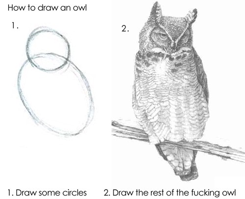
This is the post I wanted to read on the YOLO model.

You Only Look Once (YOLO)

Prior to YOLO, most object detection used sliding windows to detect objects. That basically means that an algorithm scans them image using windows of arbitrary size and checks if there is an object that it detects in there.

The problem with the sliding window is that the window size has to be determined, and in order to be able to detect objects of different sizes, there likely has to be several window sizes. Not to mention the inefficiency of having to scan over the same area multiple times. For these reasons, sliding windows make real-time object detection impractical and inflexible.

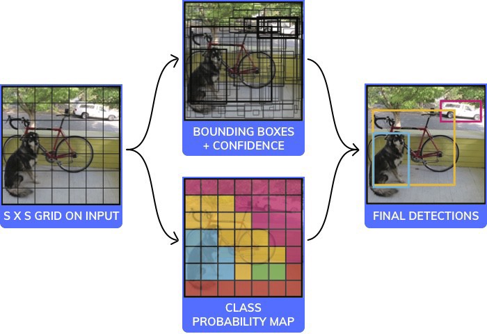
YOLO takes a different approach. The YOLO model takes the image as an input and outputs a series of coordinates for objects with their respective confidence levels and class probabilities.

The technical details of the internal workings of the model aren’t as important as understanding the output. But if you must know, here is the architecture of YOLO v1:

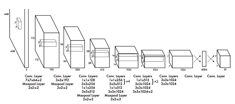
The output of the YOLO v3 model is a convolutional layer shaped (19, 19, 425). The (19, 19) are the number of squares that the image is divided into. The last unit (425) is a concatenation of each bonding box parameters, confidence intervals and class probabilities.

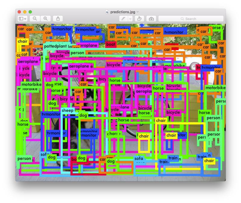
A bounding box is defined by 5 parameters: x, y, width, height and confidence value. The number of classes ( C ) will be a one-hot vector with as many classes the network was trained on (in this case 80). And the number of bounding boxes ( B ) is set at the time of training (in this case 5 — see Clustering Box Dimensions with Anchors). So the 425 size in the output layer is (B * (5 + C)) or (5 * (5 + 80)) or 425. The output can then be parsed and filtered based on class and confidence. From there, you can determine what confidence level you want to consider a match. Changing this value changes how many objects get detected. Below shows a threshold of 0:

The YOLO model has a few interesting characteristics worth diving into.

Offsets

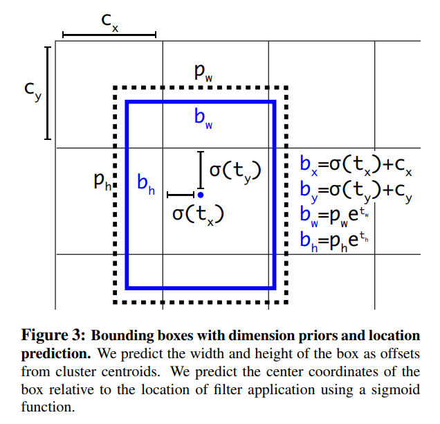
Rather than predicting the absolute coordinates of the bounding box, YOLO predicts offsets based on the grid square. It uses a sigmoid function to keep the x and y offsets between 0 and 1 with (0, 0) being the top left of the square and (1, 1) being the bottom right. Without this constraint, any bounding box center can end up at any point in the image, regardless where it came from.

Clustering Box Dimensions with Anchors

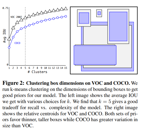
In order to assist in learning the correct dimensions for each box, YOLO provides some initial values (anchors). As mentioned above, there are 5 bounding boxes for each output. The outputs for the height and width of these values is multiplied by its respective anchors to determine final box dimensions. Here are the anchors:

array([[0.57273 , 0.677385],  
       [1.87446 , 2.06253 ],  
       [3.33843 , 5.47434 ],  
       [7.88282 , 3.52778 ],  
       [9.77052 , 9.16828 ]])

In order to determine the anchor values to use, the team used k-means clustering to calculate relative objects dimensions. They chose to use 5 clusters as a trade-off between performance and complexity.

Multi-Scale Training

As with most detection methods, YOLO uses pre-trained layers from ImageNet. Using pre-trained convolutional layers saves a lot of time as it lets a model match simple edges and basic features without starting from scratch. But most pre-trained networks are trained on images with dimensions less than 256 x 256, while YOLO uses an input 448 x 448, although this is flexible. In order to adjust for the larger image dimensions, the base pre-trained network is fine-tuned and trained for 10 epochs on the larger image size.

Since the YOLO model uses only convolutional layers, this allows the input to change. While training, the team changed input dimensions every 10 batches. Since the model down-samples by a factor of 32, they used image dimensions that are multiples of 32, with the smallest being 320 x 320 and the largest 608 x 608. This helped build a more robust model.

Training for Classification and Detection

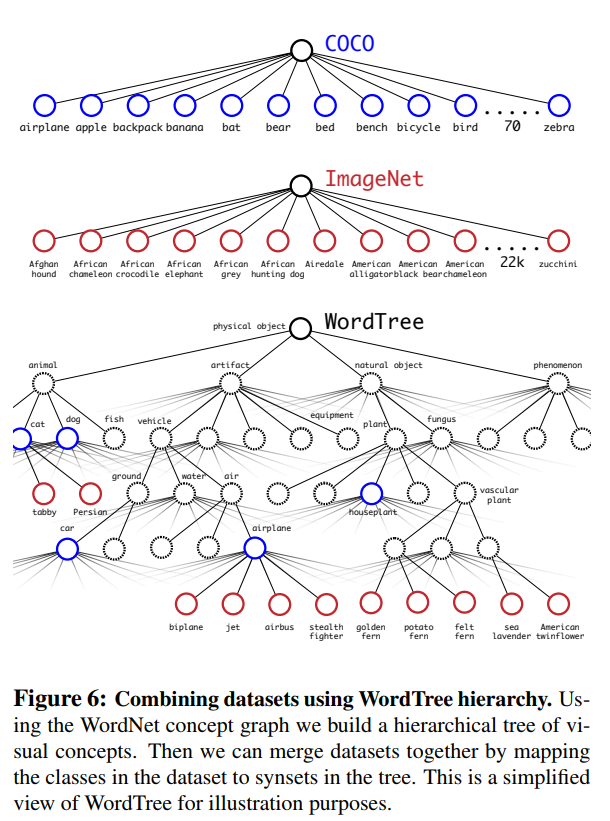
During training, the team mixed both detection and classification data sets. Different loss functions were used for each during back-propagation depending on the task. This allowed the model to learn from a much larger dataset. However, the data sets contain differences in how they label objects. For instance, detection data sets have general labels, like “dog” or “boat”. But ImageNet has more specific classifications like “Norfolk Terrier”. So the team used WordNet, a language database that structures words and how they relate. So a “Norfolk terrier” and “Yorkshire terrier” are both hyponyms of “terrier” which is a type of “hunting dog” which is a type of “dog”, and so on.

Using joint training, YOLO leans to find objects based on the COCO dataset and then classifies them using data from ImageNet.

Running YOLO

Real-time object detection requires a GPU, but detecting objects on a single image is possible on a CPU due to the efficiencies discussed. The YOLO site provides a good guide:

git clone https://github.com/pjreddie/darknetcd darknetmakewget https://pjreddie.com/media/files/yolov3.weights./darknet detect cfg/yolov3.cfg yolov3.weights data/dog.jpg

There is also a mini version with weights that are only 4.8 MB, that can supposedly run on a raspberry pi, but I haven’t gotten it to work.

If you want to hook it up to a system that does more than draws bounding boxes, you’ll have to do some work. However, if you understand how to parse the output, then it wouldn’t be difficult. Model Depot has a great guide on how to load the model and a link to the weights. I may write a future post about hooking up this model to do basic object location tracking.

Final Thoughts

The most impressive thing about YOLO is the fact that it works. The architecture makes sense to me. It has everything you’d expect in a modern image classification architecture: convolutional 2d layers, leaky relu, batch normalization and max pooling. In fact, much of the model is a fine-tuned version of Darknet-19. However, YOLO does have some creative touches.

I was impressed by the idea of dividing up the image and learning bounding box offsets and size. Also the idea of anchors to assist in learning bounding box dimensions was very clever. The larger output trades off size/complexity for an increase in speed.

But probably the most impressive thing is the loss function. The model only manages to learn what you want it to learn with an effective loss function. With simple image classification models, you can use a simple loss function like categorical cross entropy loss. But with this type of model, you have to be creative. I would argue that an effective loss function is much more important than the exact architecture. In fact, YOLO has models that are trained on fewer layers that provide similar accuracy with decreased complexity and processing power required.

Jeremy Howard from Fast.ai spoke about this as well. Determining loss functions is more of an art than a science. It pains me to think how much time the YOLO team likely spent on determining the right loss function to achieve good results. And they also had to balance how much to weight each loss when training on the two different data sets (COCO and ImageNet).

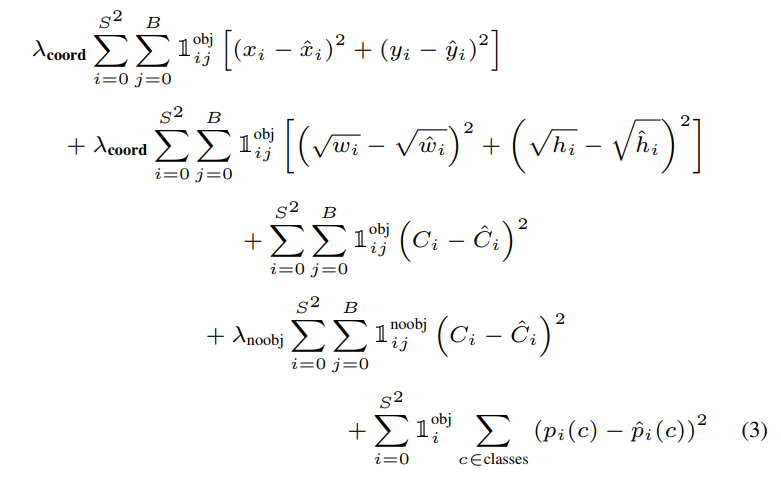
I wasn’t able to dig into the loss function from YOLO v3, but here is the loss function for version 1:

I also found the integration with WordNet particularly impressive. I’m not sure if technique was developed by the YOLO team, but it is likely to be copied going forward.

The YOLO model is very impressive in both performance and ingenuity. But most surprisingly, it is also intuitive.

By Branko Blagojevic on April 5, 2018