Stock prices are just a series of numbers. Let’s try to fit a model to those numbers. What could go wrong?
With the rise of stock market volatility in the last few months, there has been a renewed interest in the stock market. The stock market is a compelling challenge to engineers. It’s a mature market with practically unlimited depth and exceptionally low transaction costs. If you can digest the numbers and eek out a model that is just slightly better than random, you would have investors lining up to give you their money. Or you could just use leverage and exotic instruments to multiply your returns and live passively off your modest savings.
So let’s take a deep dive into predicting the stock market using data science. We’ll look at the S&P 500, an index of the largest US companies. It’s a broad index that’s a proxy for what people normally call “the market”.
We’ll want to look at the performance of S&P 500 over the last year and its daily returns. When looking at time series, it’s often useful to look at log values and log returns to normalize the values, but the last two year’s valuations aren’t so volatile, so the log values are similar to the actual values.
import datetime as dt
import matplotlib.pyplot as plt
import numpy as np
import pandas as pd

%matplotlib inline

stock = pd.read_csv("SPY.csv", index_col="Date")

cutoff = len(stock)//2

prices = pd.Series(stock.Close)
log_prices = np.log(prices)

deltas = pd.Series(np.diff(prices), index=stock.index[1:])
log_deltas = pd.Series(np.diff(log_prices), index=stock.index[1:])

latest_prices = stock.Close[cutoff:]
latest_log_prices = np.log(latest_prices)
latest_log_deltas = deltas[cutoff:]

prior_log_deltas = log_deltas[:cutoff]
prior_log_mean = np.mean(prior_log_deltas)
prior_log_std = np.std(prior_log_deltas)

f, axes = plt.subplots(ncols=2, figsize=(15,5))
prices.plot(ax=axes[0])
deltas.hist(bins=50, ax=axes[1])

f.autofmt_xdate()
f.tight_layout()
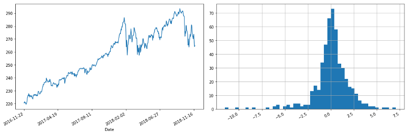
S&P 500 performance over last two years
Ideally we would like to predict log returns. Some people tried to use a neural network, specifically a recurrent neural network to predict market returns. A recurrent neural network is useful for time series data since it considers historic values. But that seems to be overkill. A neural network is unnecessarily complicated. Let’s see if we can fit a simpler model with using just random numbers!
Random Number Generator as a Model
The predict function below creates a random set of normally distributed daily returns based on the historic standard deviation and mean returns. We set the seed explicitly so we can recreate the best model and use it for forecasting.
def predict(mean, std, size, seed=None):
    """ Returns a normal distribution based on given mean, standard deviation and size"""
    np.random.seed(seed)
    return np.random.normal(loc=mean, scale=std, size=size)
The apply_returns function just applies our returns to a start price to give us a predicted stock price over time.
def apply_returns(start, returns):
    """ Applies given periodic returns """
    cur = start
    prices = [start]
    for r in returns:
        cur += r
        prices.append(cur)
    return prices
And finally, we’ll want to score the returns. There are several possible scores we can use but let’s go with mean squared error (MSE).
def score(actual, prediction):
    # mean square error
    return np.mean(np.square(actual - prediction))
It’s always useful to visualize our predictions to see how good we really are. That’s what compare is for.
def compare(prediction, actual):
    # plots a prediction over the actual series
    plt.plot(prediction, label="prediction")
    plt.plot(actual, label="actual")
    plt.legend()
Let’s see how a seed of 0 plays out.
latest_size = len(latest_log_prices)
predict_deltas = predict(prior_log_mean, prior_log_std, latest_size, seed = 0)
start = latest_log_prices[0]
prediction = apply_returns(start, predict_deltas)
print("MSE: {:0.08f}".format(score(latest_log_prices, prediction)))
compare(prediction=prediction, actual=latest_log_prices.values)

MSE: 0.00797138
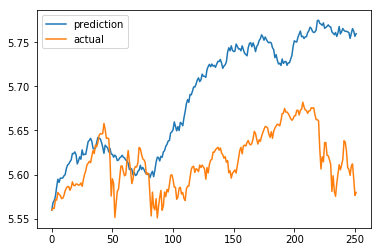
Prediction using a seed of 0
It’s not great but it’s a start. Our model predicted the rise early on this year, but it definitely overshot. This is the point where we’ll want to tune our model’s seed value to better predict the actual market.
predict_partial = lambda s: predict(mean = prior_log_deltas_mean, std = prior_log_deltas_std, size = latest_size, seed = s)
def find_best_seed(actual, predict_partial, score, start_seed, end_seed):
    best_so_far = None
    best_score = float("inf")
    start = actual[0]
    for s in range(start_seed, end_seed):
        print('r{} / {}'.format(s, end_seed), end="")
        predict_deltas = predict_partial(s)
        predict_prices = apply_returns(start, predict_deltas)
        predict_score = score(actual, predict_prices)
        if predict_score < best_score:
            best_score = predict_score
            best_so_far = s
    return best_so_far, best_score

best_seed, best_score = find_best_seed(latest_log_prices, predict_partial, score, start_seed=0, end_seed=500000)
print("best seed: {} best MSE: {:0.08f}".format(best_seed, best_score))

best seed: 68105 best MSE: 0.00035640
After 500k trials, we decreased our MSE to 0.0003564 from 0.00797! That’s a huge improvement.
Historic performance is nice, but we really want to see what our magic seed says for the next few months.
returns = predict(mean=prior_log_deltas_mean, std=prior_log_deltas_std, size=400, seed=best_seed)

prediction = apply_returns(start, returns)
compare(prediction, latest_log_prices.values)

compare(prediction, log_prices.values)
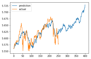
Our model using the best seed
There you have it. According to our model, the market should begin to pick up and reach new heights by the end of the year.
p-Hacking
Statistical measures such as t-tests and p-values are useful in evaluating relationships between data, but they can be hacked. Anyone can get a statistically significant result by chance if they run enough tests. And you don’t have to report the number of trials and considerations you made prior to achieving a statistically significant result.

There has been a bit of a reproducability crisis where some scientists were not able to replicate some key experiments:
In August, the journal Science published the results of an ambitious initiative called the Reproducibility Project, a collaborative effort coordinated by the nonprofit Center for Open Science. Participants attempted to replicate 100 experimental and correlational psychology studies that had been published in three prominent psychology journals.
The results — widely reported in the media — were sobering. Just 39 of the studies were successfully replicated (Science, 2015). Psychology, it seemed, had a credibility problem.
I suspect that much of the reason is that researchers conducted a large number of trials prior to publishing statistically significant results. Or they change various parameters during the trial. This is called garden of the forking paths and is not always deliberate.
Researcher degrees of freedom can lead to a multiple comparisons problem, even in settings where researchers perform only a single analysis on their data. The problem is there can be a large number of potential comparisons when the details of data analysis are highly contingent on data, without the researcher having to perform any conscious procedure of fishing or examining multiple p-values
Economic and financial forecasting is particularly susceptible to these biases. I’ve heard stories economists often claim that the N month lag of factor X is an indicator of Y. Why the N month lag? Well, lags of 1 — (N-1) hadn’t worked out.
Avoiding p-Hacking
A good way to avoid p-hacking in your own research is to be honest with yourself from the onset. Think through and document everything you want to test. If you want to test 20 different factors, specify the factors before you start testing and consider all 20 factors when evaluating your metrics.
But most importantly, ask yourself what your model is doing. Neural networks sometimes have the reputations of being black boxes, and in a sense they are. But you should review each step critically. If you’re doing image recognition, observe each layer’s activations and see roughly what the layer is activating based on. If you’re doing reinforcement learning to play games, look at contrived scenarios and see if you can understand roughly how the logic works. If you’re doing natural language processing, consider word vectors in relation to synonyms, antonyms and related words.
And if you’re doing stock market analysis, ask yourself what you’re actually trying to get out of the model. Why is the Nth lag of some factor a predictor? Why do the prior returns impact the future returns? Why are you considering only the N latest returns? Why are you predicting a return periodicity of [daily, hourly, minute]? Why did you consider the time period from X to Y? Why did you validate up to Z?
Just feeding stock deltas into a recurrent neural network may achieve the goal of being able to decrease the loss, but with an explanation, you may as well be fitting the values to a random number generator.
By Branko Blagojevic on November 29, 2018