Optimize your fantasy football picks with a linear regression in just a few lines of code.

Using a regression to predict fantasy football performance is easier than you think in R. With a few lines of code, you can predict player performance and optimize your lineup.

In a prior post, I wrote about using linear programming to optimize your fantasy football picks. Linear programming ensures you pick the best lineup based on some points projections and constraints (e.g. position and salary constraints). In that post, I had used average points this year as a proxy for points, but obviously that’s a flawed method. For instance, the players may do better or worse depending on their opponent. In this post, I’ll build on the optimization and design an actual strategy based on historic information. All the code is available here.

I re-wrote the linear optimization in R. If you’re used to numerical analysis in python using pandas and numpy, R should be quick to pick up. Much of the pandas DataFrame api was modeled after R data frames. I found Practical Statistics for Data Scientists by O’Reilly to be a good resource. It’s a good combination of explaining statistical concepts and usage. Another resource I would recommend that is in Python is Data Science from Scratch. It implements the basic tools of any data scientist from scratch and teaches the concepts along the way.

Fantasy Football

The details of how fantasy football scoring works is not important. Each player is awarded points based on how they performed in real life. For instance, 1 point per 25 passing yards, 4 points for a passing touchdown, etc. I use DraftKings (DK) points scoring system. As a side-note, Fantasy Football is big money with plenty of sharks. The competitions are very competitive and DraftKings take a healthy cut. There is a lot of variance as well, so a prudent strategy would include making a large number of smaller wagers and hoping for a statistical edge. In that respect, there is no optimal pool. I haven’t studied the actual market enough, but I doubt simple statistical methods would give you an edge in public competitions. But if you do want to dabble, use can use my referral to sign up or not.

Downloading History and Available Players in R

I downloaded all the DraftKings historical information from RotoGuru. They store the DK history in an easily digestible csv format. The base url is below, after which you swap out the WEEK and YEAR with their respective values.

HISTORY_BASE_URL <- "[http://rotoguru1.com/cgi-bin/fyday.pl?game=dk&scsv=1&week=WEEK&year=YEAR](http://rotoguru1.com/cgi-bin/fyday.pl?game=dk&scsv=1&week=WEEK&year=YEAR)"

The file history.R has functions that download, aggregate and update the history. The function updateHistory downloads the DK history from 2014 to today.

If you want to save or update the history retrieved earlier, just pass in a data frame:

# downloads history from 2014 - today  
history <- updateHistory()

# update history  
history <- updateHistory(history)

# saves the history (default "history.csv")  
saveHistory(history, "history.csv")

Here is the history:

Running a Regression

Before I run the regression, I’ll want to add some fields I think would be useful. The function enrichHistory adds a few fields like date and games. The games value says how many games the player has played in this year. I may want to avoid players that don’t have much of a history in my regression. In the example below, I filter the data to include only the last two years of history and players that played 3 or more games in a year.

# Get and enrich history  
h <- getLatestHistory()  
h <- updateHistory(h)  
h <- enrichHistory(h)

# Run a regression based on history  
h2016 <- h[(as.numeric(as.character(h$year)) >= 2016) & (h$games > 3),]

To get an fair estimate of how the model is doing, I separate the data into a training and test set.

trainingRowIndex <- sample(1:nrow(h2016), 0.8*nrow(h2016))  
trainingData <- h2016[trainingRowIndex, ]  
testData  <- h2016[-trainingRowIndex, ]

Finally, I run the regression

fit <- lm(dk.points ~ displayName + team + year + h.a + week + pos, data = trainingData)

summary(fit)

The number of coefficients in the model is equal to the sum of the number of unique players, teams, years, home/away, weeks and positions. Note that the intercept is 11.23 and a good chunk of the players don’t have a statistically significant coefficient. For instance, Adam Humphries is more or less the average wide for wide received for Tampa.

How did the model do? Mean square error (MSE) tells us the average of the error (actual − forecast).

mean((predict(fit, trainingData) - trainingData$dk.points) ^ 2)  
35.00807

mean((predict(fit, testData) - testData$dk.points) ^ 2)  
36.66413

That means on the data the model has seen, it’s off by around +/- 5.9 points (square root of 34). But for the data our model hasn’t seen, it’s off by +/- 6 points. Your numbers may be different since we used a random train/test set. You may also note that there is a warning:

Warning message:  
In predict.lm(fit, testData) :  
  prediction from a rank-deficient fit may be misleading

There is a good stack overflow answer for this, but the short answer is that there is collinear covariates which means our variables are correlated. To build a more serious model you’d probably want to address this.

Predicting Performance on Available Players

Now that I have a model, I can use it to predict how the vailable players will do.

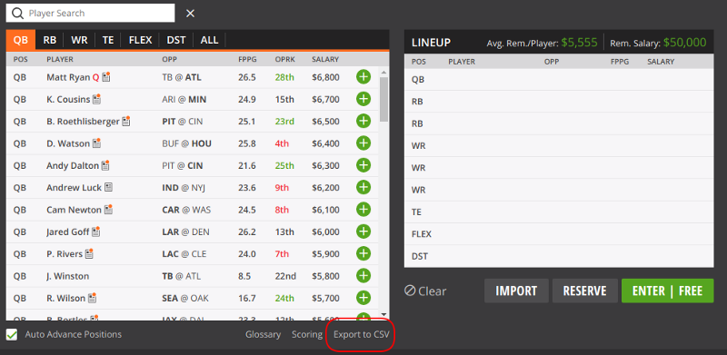
Unfortunately, RotoGuru does not have the current available line-up available, or I wasn’t able to find it. Also, depending on the contest, your line-up may exclude some players (e.g. players playing on weekday games). To get the available line-up for your contest, you need a weeks_id. You can get your weeks_id from the contest page by checking the link to Export to CSV.

The file available.R has functions that allow you to retrieve your available line up. There are some differences between how RotoGuru shows players and stats and how DraftKings does, so we need to transform the available format to history format (e.g. Bob Smith vs Smith, Bob or Atlanta vs Falcons).

a <- getLatestAvailable(WEEKS_ID)  
ah <- availableToHistory(a, WEEK, YEAR, history=h2016)

I pass in the history to my availableToHistory function since I want to do a fuzzy match on displayName. For instance, our history may have Allen Robinson II while the available has Allen Robinson.

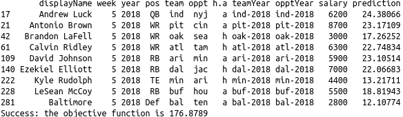
Since I filtered out some players from our history and some available players may be new, my regression won’t be able to predict every player. For example, based on my history, A.J. McCarron only played one game in 2016, 3 games in 2017 and 1 game in 2018, so he was excluded from our regression. Since the model never saw his name before, it cannot predict how he will do. Before I predict, I need to filter out those names.

ahFiltered <- ah[(ah$displayName %in% h2016$displayName),]

Finally, I can predict and solve for the optimal team based on my prediction and constraints:

ahFiltered$prediction <- predict(fit, ahFiltered)  
solve(ahFiltered)

Again, your line-up may be different since the regression was trained on a random sample of the training set.

Issues with the Model

Here are some of the main issues with the model.

Time variables are factors

The model treats year and week as factors. That means there is no relationship between weeks. Week 1 is its own variable, week 2 is its own variable, and so on. In reality, we would want a time component and treat this as a time series.

Variables are independent

There is a variable for the year which is applied uniformly to all predictions for that year. Maybe there was something special about the one year that would affect all players, or maybe there were some rule changes or extreme weather all year, but this is unlikely. The year is more relevant to the player or team. One team might have done very well in 2016, but less well in 2017. Or one player could have had a good year.

There are no interactions between variables

Every variable is independent which is a problem. For instance, a team may have a strong pass defense. So a wide receiver would be negatively impacted when facing this team. Right now, we evaluate the player and the opponent independently. Ideally, we would decompose players into a vector. For instance, consider a simple two factor model for the player and opponent:

player = [running, passing]
oppt = [running, passing]
performance = player * oppt

Strong running player, weak running defense

player = [1.0, 0.3]
oppt = [1.0, 0.5]
performance = [1.0, 0.15]

Strong running player, strong running defense

player = [1.0, 0.3]
oppt = [0.5, 0.5]
performance = [0.5, 0.15]

Weak running player, strong running defense

player = [0.5, 0.3]
oppt = [0.5, 0.5]
performance = [0.25, 0.15]

In the example above a high player number means strong while a high oppt number means weak. So the product of the two vectors determines performance.

Of course you wouldn’t manually pick factors for each variable. You would just tell the model, imagine each player and team is a series of 2 random numbers, solve so that the sum-product of the two vectors is correlated to the points the player actually scores.

Too much variability

I ran the model a few times and got significantly different results due to the sample chosen. Ideally, you would want to use a k-folds or other method to choose a model. You would also want to more closely examine some predictions and biases of the model.

Final thoughts

A regression is a good start but it is very limited. I like the idea of a factor model, which I may implement in a future post. I’m not entirely convinced that fantasy football is stable enough to make a meaningful model, but there is a fair amount of data out there that it’s worth playing around with. I also haven’t studied the competitive DraftKing competitions but my initial impression that the people participating are very strong and use much more sophisticated models.

By Branko Blagojevic on October 11, 2018